graph TD
    A["The"] --> B["<b>nice</b> (0.5)"]
    A --> C["dog (0.4)"]
    A --> D["car (0.1)"]
    B --> E["<b>woman</b> (0.4)"]
    B --> F["day (0.3)"]
    B --> G["house (0.3)"]

    style B fill:#56cc9d,stroke:#333,color:#fff
    style E fill:#56cc9d,stroke:#333,color:#fff
    style C fill:#f8f9fa,stroke:#ccc
    style D fill:#f8f9fa,stroke:#ccc
    style F fill:#f8f9fa,stroke:#ccc
    style G fill:#f8f9fa,stroke:#ccc
Decoding Methods for Text Generation with LLMs
A hands-on comparison of greedy search, beam search, sampling, top-k, top-p, and contrastive search using small pretrained models
Keywords: decoding methods, text generation, greedy search, beam search, top-k sampling, top-p sampling, nucleus sampling, contrastive search, temperature, GPT-2, transformers, LLM inference
Introduction
When a pretrained language model generates text, it produces a probability distribution over the entire vocabulary at each step. The decoding method determines how the next token is selected from that distribution. This choice has a dramatic effect on output quality — the same model can produce boring repetitive text or creative human-like prose, depending entirely on the decoding strategy.
This article provides a practical, hands-on comparison of six common decoding methods using GPT-2 (124M parameters) — a small model that runs comfortably on CPU. All code examples use the Hugging Face transformers library and can be reproduced on any machine.
If you are new to running LLMs locally, check out Run LLM Locally with Ollama for a beginner-friendly setup guide. For deploying models at scale, see Deploying and Serving LLM with vLLM and Deploying and Serving LLM with Llama.cpp.
How Auto-Regressive Generation Works
All decoder-only LLMs (GPT-2, Llama, Mistral, Phi, etc.) generate text one token at a time. The probability of a word sequence is decomposed as:
P(w_{1:T} | W_0) = \prod_{t=1}^{T} P(w_t | w_{1:t-1}, W_0)
where W_0 is the initial prompt (context) and T is the generated sequence length. Generation stops when the model emits an end-of-sequence (EOS) token or a maximum length is reached.
The key question is: how do we pick w_t from P(w_t | w_{1:t-1}) at each step? That is exactly what a decoding method defines.
Setup
Install the required library and load the model:
pip install transformers torchfrom transformers import AutoModelForCausalLM, AutoTokenizer, set_seed
import torch
device = "cuda" if torch.cuda.is_available() else "cpu"
tokenizer = AutoTokenizer.from_pretrained("gpt2")
model = AutoModelForCausalLM.from_pretrained(
"gpt2", pad_token_id=tokenizer.eos_token_id
).to(device)
prompt = "Artificial intelligence is"
inputs = tokenizer(prompt, return_tensors="pt").to(device)We use GPT-2 (124M parameters) throughout — small enough to run on CPU, yet large enough to demonstrate clear differences between decoding strategies.
1. Greedy Search
Greedy search is the simplest strategy. At each step, it selects the token with the highest probability:
w_t = \arg\max_w P(w | w_{1:t-1})
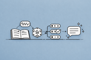
Greedy search always follows the green path — picking the single highest-probability token at each step. Result: “The nice woman” (0.5 x 0.4 = 0.20). It misses “The dog has” (0.4 x 0.9 = 0.36).
output = model.generate(**inputs, max_new_tokens=60)
print(tokenizer.decode(output[0], skip_special_tokens=True))
Pros:
- Fast and deterministic.
- Good for short, factual outputs.
Cons:
- Quickly falls into repetitive loops — the model keeps generating the same phrases.
- Misses high-probability sequences hidden behind lower-probability initial tokens.
Greedy search is the default in transformers when no other parameters are specified.
2. Beam Search
Beam search keeps track of the top n most likely partial sequences (called beams) at each step, then selects the sequence with the highest overall probability. It reduces the risk of missing good sequences that greedy search would overlook.
graph TD
    A["The"] --> B["nice (0.5)"]
    A --> C["dog (0.4)"]
    B --> E["woman (0.4)<br/>path: 0.20"]
    B --> F["day (0.3)<br/>path: 0.15"]
    C --> G["<b>has (0.9)</b><br/><b>path: 0.36</b>"]
    C --> H["runs (0.05)<br/>path: 0.02"]

    style B fill:#6cc3d5,stroke:#333,color:#fff
    style C fill:#6cc3d5,stroke:#333,color:#fff
    style G fill:#56cc9d,stroke:#333,color:#fff
    style E fill:#f8f9fa,stroke:#ccc
    style F fill:#f8f9fa,stroke:#ccc
    style H fill:#f8f9fa,stroke:#ccc
With num_beams=2, both “nice” and “dog” are kept (blue). At the next step, all continuations are scored and the best overall path — “The dog has” (0.36) — wins (green).
output = model.generate(
    **inputs,
    max_new_tokens=60,
    num_beams=5,
    no_repeat_ngram_size=2,
    early_stopping=True
)
print(tokenizer.decode(output[0], skip_special_tokens=True))
Key parameters:
| Parameter | Description |
|---|---|
num_beams |
Number of beams to track (higher = more exploration, slower) |
no_repeat_ngram_size |
Prevents any n-gram from appearing twice |
early_stopping |
Stops when all beams reach the EOS token |
num_return_sequences |
Return multiple candidate sequences |
Pros:
- Finds higher-probability sequences than greedy search.
- Effective for tasks with predictable output length (translation, summarization).
Cons:
- Still suffers from repetition without n-gram penalties.
- Produces text that is too predictable and lacks diversity for open-ended generation.
- Slower than greedy search due to tracking multiple beams.
3. Pure Sampling
Sampling randomly picks the next token according to its probability distribution:
w_t \sim P(w | w_{1:t-1})
This introduces randomness, breaking the repetition patterns of deterministic methods.
graph TD
    A["Vocabulary distribution"] --> B["nice — 50%"]
    A --> C["dog — 30%"]
    A --> D["car — 10%"]
    A --> E["the — 5%"]
    A --> F["banana — 3%"]
    A --> G["... — 2%"]
    D -.->|"🎲 randomly selected"| H["Next token: car"]

    style D fill:#ffce67,stroke:#333
    style H fill:#ffce67,stroke:#333
    style B fill:#f8f9fa,stroke:#ccc
    style C fill:#f8f9fa,stroke:#ccc
    style E fill:#f8f9fa,stroke:#ccc
    style F fill:#f8f9fa,stroke:#ccc
    style G fill:#f8f9fa,stroke:#ccc
Every token in the vocabulary has a chance proportional to its probability. Even low-probability tokens like “car” (10%) can be selected, which adds diversity but also risk of incoherence.
set_seed(42)
output = model.generate(
    **inputs,
    max_new_tokens=60,
    do_sample=True,
    top_k=0  # disable top-k to use full vocabulary
)
print(tokenizer.decode(output[0], skip_special_tokens=True))
Pros:
- Eliminates repetition.
- Produces diverse, creative outputs.
Cons:
- Can produce incoherent or nonsensical text because low-probability (weird) tokens still have a chance of being selected.
Pure sampling is rarely used in practice — the variants below (temperature, top-k, top-p) are used to make it more controlled.
4. Temperature Scaling
Temperature \tau reshapes the probability distribution before sampling. It is applied to the logits before the softmax:
P(w_i) = \frac{\exp(z_i / \tau)}{\sum_j \exp(z_j / \tau)}
graph TD
    subgraph low["Low temp (τ=0.3) — Sharp"]
        direction TB
        a1["nice — 80%"]
        a2["dog — 15%"]
        a3["car — 5%"]
    end
    subgraph mid["Normal (τ=1.0) — Original"]
        direction TB
        b1["nice — 50%"]
        b2["dog — 30%"]
        b3["car — 20%"]
    end
    subgraph high["High temp (τ=2.0) — Flat"]
        direction TB
        c1["nice — 35%"]
        c2["dog — 33%"]
        c3["car — 32%"]
    end

    style low fill:#56cc9d,stroke:#333,color:#fff
    style mid fill:#6cc3d5,stroke:#333,color:#fff
    style high fill:#ff7851,stroke:#333,color:#fff
Low temperature concentrates probability on the top token (more deterministic). High temperature flattens the distribution toward uniform (more random). At τ→0, it becomes greedy search.
| Temperature | Effect |
|---|---|
| \tau < 1 | Sharpens the distribution — high-probability tokens become even more likely. Output is more focused and deterministic. |
| \tau = 1 | No change — original distribution. |
| \tau > 1 | Flattens the distribution — low-probability tokens get a bigger share. Output is more random and creative. |
| \tau \to 0 | Equivalent to greedy search. |
set_seed(42)
# Low temperature → more focused
output = model.generate(
    **inputs,
    max_new_tokens=60,
    do_sample=True,
    temperature=0.3,
    top_k=0
)
print("Low temp:", tokenizer.decode(output[0], skip_special_tokens=True))

set_seed(42)
# High temperature → more creative
output = model.generate(
    **inputs,
    max_new_tokens=60,
    do_sample=True,
    temperature=1.5,
    top_k=0
)
print("High temp:", tokenizer.decode(output[0], skip_special_tokens=True))
Temperature is typically used in combination with top-k or top-p, not alone. Common values range from 0.3 (factual) to 1.0 (creative).
5. Top-K Sampling
Top-K sampling (Fan et al., 2018) filters the vocabulary to only the K most likely tokens, then redistributes the probability mass among them.
graph LR
    A["Full vocabulary<br/>(50,257 tokens)"] --> B["Sort by<br/>probability"]
    B --> C["Keep top K=5<br/>tokens only"]
    C --> D["Renormalize<br/>probabilities"]
    D --> E["🎲 Sample from<br/>filtered set"]

    style A fill:#f8f9fa,stroke:#333
    style B fill:#6cc3d5,stroke:#333,color:#fff
    style C fill:#ffce67,stroke:#333
    style D fill:#56cc9d,stroke:#333,color:#fff
    style E fill:#78c2ad,stroke:#333,color:#fff
graph TD
    subgraph kept["Kept — Top K=5"]
        T1["nice — 0.30"]
        T2["dog — 0.25"]
        T3["big — 0.20"]
        T4["old — 0.15"]
        T5["red — 0.10"]
    end
    subgraph removed["Removed"]
        T6["the — 0.04"]
        T7["a — 0.02"]
        T8["banana — 0.001"]
        T9["... 50K+ tokens"]
    end

    style kept fill:#56cc9d,stroke:#333,color:#fff
    style removed fill:#f8f9fa,stroke:#ccc
Top-K keeps a fixed number of candidates regardless of how the probability is distributed. The removed tail tokens can never be selected.
set_seed(42)
output = model.generate(
    **inputs,
    max_new_tokens=60,
    do_sample=True,
    top_k=50
)
print(tokenizer.decode(output[0], skip_special_tokens=True))
How it works:
- Compute the probability distribution over the full vocabulary.
- Keep only the top K tokens.
- Renormalize probabilities among these K tokens.
- Sample from the filtered distribution.
Pros:
- Eliminates nonsensical low-probability tokens.
- GPT-2 used top-k=40 and became famous for generating coherent stories.
Cons:
- Fixed K does not adapt to the shape of the distribution. When the model is very confident (sharp distribution), K=50 may include garbage tokens. When the model is uncertain (flat distribution), K=50 may exclude reasonable candidates.
6. Top-p (Nucleus) Sampling
Top-p sampling (Holtzman et al., 2019) dynamically selects the smallest set of tokens whose cumulative probability exceeds a threshold p.
graph TD
    subgraph confident["Confident distribution — only 3 tokens needed"]
        direction LR
        C1["nice — 0.60"] --> C2["dog — 0.25"] --> C3["big — 0.10"]
    end
    subgraph uncertain["Uncertain distribution — 7 tokens needed"]
        direction LR
        U1["nice — 0.18"] --> U2["dog — 0.16"] --> U3["big — 0.14"] --> U4["old — 0.13"] --> U5["red — 0.12"] --> U6["the — 0.11"] --> U7["a — 0.10"]
    end

    P["p = 0.92"] --> confident
    P --> uncertain

    style confident fill:#56cc9d,stroke:#333,color:#fff
    style uncertain fill:#6cc3d5,stroke:#333,color:#fff
    style P fill:#ffce67,stroke:#333
Top-p adapts the candidate set size dynamically. When the model is confident (sharp distribution), few tokens suffice. When uncertain (flat distribution), more tokens are included. This is the key advantage over fixed Top-K.
set_seed(42)
output = model.generate(
    **inputs,
    max_new_tokens=60,
    do_sample=True,
    top_p=0.92,
    top_k=0  # disable top-k to let top-p work alone
)
print(tokenizer.decode(output[0], skip_special_tokens=True))
How it works:
- Sort tokens by probability (descending).
- Cumulate probabilities until the sum exceeds p.
- Discard all tokens beyond that cutoff.
- Renormalize and sample.
Pros:
- Adapts dynamically — uses fewer tokens when the model is confident, more tokens when it is uncertain.
- Generally produces more fluent and coherent text than top-k for open-ended generation.
Cons:
- Still non-deterministic — results vary across runs.
Combining top-k and top-p is a common practice: top-k first removes the long tail, then top-p refines the selection dynamically.
set_seed(42)
output = model.generate(
    **inputs,
    max_new_tokens=60,
    do_sample=True,
    top_k=50,
    top_p=0.95,
    temperature=0.8
)
print(tokenizer.decode(output[0], skip_special_tokens=True))
7. Contrastive Search
Contrastive search (Su et al., NeurIPS 2022) is a newer deterministic method designed to produce human-level text without the repetition of greedy/beam search and without the incoherence of sampling.
graph TD
    A["Top-K candidates<br/>(k=4)"] --> B["Candidate: nice"]
    A --> C["Candidate: dog"]
    A --> D["Candidate: big"]
    A --> E["Candidate: old"]

    B --> F["Model confidence: 0.50"]
    B --> G["Degeneration penalty: 0.85<br/>(similar to context)"]
    F --> H["Score = (1-α)·0.50 − α·0.85"]

    C --> I["Model confidence: 0.30"]
    C --> J["Degeneration penalty: 0.20<br/>(different from context)"]
    I --> K["Score = (1-α)·0.30 − α·0.20 ✅"]

    style K fill:#56cc9d,stroke:#333,color:#fff
    style H fill:#f8f9fa,stroke:#ccc
    style B fill:#ff7851,stroke:#333,color:#fff
    style C fill:#56cc9d,stroke:#333,color:#fff
“nice” has higher probability but is too similar to previous context (high penalty). “dog” is less probable but brings new information (low penalty), so it wins. This prevents degenerate repetition while staying coherent.
At each step, it selects the token that maximizes:
(1 - \alpha) \times \underbrace{P(v | x_{<t})}_{\text{model confidence}} - \alpha \times \underbrace{\max_{j < t} \cos(h_v, h_{x_j})}_{\text{degeneration penalty}}
where:
- Model confidence: the probability assigned by the language model (keeps the text coherent).
- Degeneration penalty: the maximum cosine similarity between the candidate token’s representation and all previous token representations (prevents repetition).
- \alpha controls the trade-off. When \alpha = 0, it reduces to greedy search.
output = model.generate(
    **inputs,
    max_new_tokens=60,
    penalty_alpha=0.6,
    top_k=4
)
print(tokenizer.decode(output[0], skip_special_tokens=True))
Key parameters:
| Parameter | Description |
|---|---|
penalty_alpha |
The \alpha hyperparameter (typically 0.5–0.6) |
top_k |
Number of candidate tokens considered at each step (typically 4–10) |
Pros:
- Deterministic — same input always produces the same output.
- Generates remarkably fluent and coherent text, often approaching human quality.
- Avoids repetition without needing n-gram penalties.
Cons:
- Slower than greedy search (requires computing token representations at each step).
- Less creative/diverse than sampling-based methods.
Comparison Summary
| Method | Deterministic | Repetition | Coherence | Diversity | Speed |
|---|---|---|---|---|---|
| Greedy Search | Yes | High | Medium | Low | Fast |
| Beam Search | Yes | Medium* | Medium-High | Low | Medium |
| Pure Sampling | No | Low | Low | High | Fast |
| Top-K Sampling | No | Low | Medium-High | Medium-High | Fast |
| Top-p Sampling | No | Low | High | Medium-High | Fast |
| Contrastive Search | Yes | Low | Very High | Medium | Slow |
*with n-gram penalty enabled
When to Use What
- Factual / deterministic tasks (translation, summarization, code generation): Use beam search with n-gram penalty, or contrastive search.
- Creative / open-ended generation (storytelling, dialogue, brainstorming): Use top-p + top-k + temperature sampling.
- Maximum quality on open-ended text: Try contrastive search — it often produces the most human-like output from off-the-shelf models.
- Quick prototyping / debugging: Greedy search is fast and reproducible; useful for sanity-checking that the model works.
Full Working Example
Below is a complete script that generates text using all six methods for side-by-side comparison:
from transformers import AutoModelForCausalLM, AutoTokenizer, set_seed
import torch

device = "cuda" if torch.cuda.is_available() else "cpu"
tokenizer = AutoTokenizer.from_pretrained("gpt2")
model = AutoModelForCausalLM.from_pretrained(
    "gpt2", pad_token_id=tokenizer.eos_token_id
).to(device)

prompt = "The future of artificial intelligence is"
inputs = tokenizer(prompt, return_tensors="pt").to(device)
max_tokens = 80

print("=" * 70)
print("PROMPT:", prompt)
print("=" * 70)

# 1. Greedy Search
output = model.generate(**inputs, max_new_tokens=max_tokens)
print("\n[Greedy Search]")
print(tokenizer.decode(output[0], skip_special_tokens=True))

# 2. Beam Search
output = model.generate(
    **inputs, max_new_tokens=max_tokens,
    num_beams=5, no_repeat_ngram_size=2, early_stopping=True
)
print("\n[Beam Search (5 beams, no repeat 2-gram)]")
print(tokenizer.decode(output[0], skip_special_tokens=True))

# 3. Pure Sampling
set_seed(42)
output = model.generate(
    **inputs, max_new_tokens=max_tokens,
    do_sample=True, top_k=0
)
print("\n[Pure Sampling]")
print(tokenizer.decode(output[0], skip_special_tokens=True))

# 4. Top-K Sampling
set_seed(42)
output = model.generate(
    **inputs, max_new_tokens=max_tokens,
    do_sample=True, top_k=50
)
print("\n[Top-K Sampling (k=50)]")
print(tokenizer.decode(output[0], skip_special_tokens=True))

# 5. Top-p Sampling
set_seed(42)
output = model.generate(
    **inputs, max_new_tokens=max_tokens,
    do_sample=True, top_p=0.92, top_k=0
)
print("\n[Top-p Sampling (p=0.92)]")
print(tokenizer.decode(output[0], skip_special_tokens=True))

# 6. Contrastive Search
output = model.generate(
    **inputs, max_new_tokens=max_tokens,
    penalty_alpha=0.6, top_k=4
)
print("\n[Contrastive Search (alpha=0.6, k=4)]")
print(tokenizer.decode(output[0], skip_special_tokens=True))
Conclusion
The decoding method is just as important as the model itself for text generation quality. Greedy and beam search are simple and deterministic but prone to repetition. Sampling methods (top-k, top-p) introduce randomness for creative diversity but can sacrifice coherence. Contrastive search offers a compelling middle ground — deterministic, fluent, and repetition-free.
For small models like GPT-2, the choice of decoding method has an outsized impact because the model has less capacity to self-correct. Experimenting with different strategies and their hyperparameters is essential to get the best output for your specific use case.
References
- Patrick von Platen, How to generate text: using different decoding methods for language generation with Transformers, Hugging Face Blog, 2020 (updated 2023).
- Yixuan Su and Tian Lan, Generating Human-level Text with Contrastive Search in Transformers, Hugging Face Blog, 2022.
- Fan et al., Hierarchical Neural Story Generation, ACL 2018 — introduced Top-K sampling.
- Holtzman et al., The Curious Case of Neural Text Degeneration, ICLR 2020 — introduced Top-p (nucleus) sampling.
- Su et al., A Contrastive Framework for Neural Text Generation, NeurIPS 2022 — introduced contrastive search.
- Hugging Face, Generation Strategies Documentation.
Read More
- Experiment with different small models: DistilGPT-2 (82M), Phi-2 (2.7B), or Qwen2.5-0.5B.
- Combine decoding methods with fine-tuned models for domain-specific generation.
- Serve your model locally with Ollama or llama.cpp and control decoding via API parameters.
- Explore advanced techniques: speculative decoding, min-p sampling, and classifier-free guidance.