graph LR
    U["User Query"] --> QR["Query Router"]
    QR --> SC["Semantic Cache"]
    SC -->|Cache Hit| A["Answer"]
    SC -->|Cache Miss| HS["Hybrid Search<br/>(Dense + Sparse)"]
    HS --> RR["Reranker"]
    RR --> LLM["LLM Generation"]
    LLM --> A
    LLM --> SC2["Cache Write"]

    subgraph Observability
        O["Tracing / Metrics"]
    end

    QR -.-> O
    HS -.-> O
    LLM -.-> O

    style U fill:#4a90d9,color:#fff,stroke:#333
    style QR fill:#e74c3c,color:#fff,stroke:#333
    style SC fill:#f5a623,color:#fff,stroke:#333
    style HS fill:#9b59b6,color:#fff,stroke:#333
    style RR fill:#27ae60,color:#fff,stroke:#333
    style LLM fill:#C8CFEA,color:#fff,stroke:#333
    style A fill:#1abc9c,color:#fff,stroke:#333
    style SC2 fill:#f5a623,color:#fff,stroke:#333
    style O fill:#e67e22,color:#fff,stroke:#333
    style Observability fill:#F2F2F2,stroke:#D9D9D9
RAG in Production: Scaling, Caching, and Observability
Vector database selection, semantic caching, query routing, hybrid search, monitoring, and cost optimization for enterprise RAG deployments
Keywords: RAG production, vector database scaling, semantic caching, GPTCache, query routing, hybrid search, observability, Langfuse, LangSmith, cost optimization, latency, sharding, replication, monitoring, enterprise RAG, Qdrant, Pinecone, pgvector
Introduction
Getting a RAG prototype running takes an afternoon. Getting it to serve 10,000 concurrent users at sub-second latency with 99.9% uptime while keeping costs under control — that’s where the real engineering begins.
Production RAG systems face challenges that never appear in demos: vector database queries slow down as collections grow past millions of documents, LLM API costs balloon when every query triggers a full retrieval-and-generation cycle, routers must decide which index or strategy to use for each query type, and when something breaks at 3 AM, you need observability to diagnose it fast.
This article covers the six pillars of production RAG: vector database scaling, semantic caching, query routing, hybrid search tuning, observability and monitoring, and cost optimization. Each section includes practical code with LlamaIndex and LangChain.
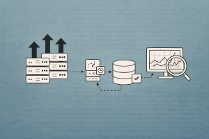
The Production RAG Architecture
Every component in the diagram above adds latency, cost, and failure modes. Production engineering is about minimizing all three simultaneously.
Pillar 1: Vector Database Selection and Scaling
The vector store is the heart of your RAG system — it determines retrieval latency, throughput ceiling, and operational complexity. The choice that works for 10K documents is rarely the right one for 10M.
Vector Database Comparison for Production
| Database | Deployment | Hybrid Search | Sharding | Replication | Filtering | Best For |
|---|---|---|---|---|---|---|
| Qdrant | Self-hosted / Cloud | Yes | Auto | Yes (RF=2+) | HNSW-integrated | Production, complex filters |
| Pinecone | Managed | Yes | Serverless | Built-in | Metadata | Zero-ops, fast time-to-value |
| Weaviate | Self-hosted / Cloud | Yes | Auto | Yes | Module-based | Multi-tenant enterprise |
| Milvus | Self-hosted / Zilliz | Yes | Auto | Yes | Attribute | Billion-scale datasets |
| pgvector | PostgreSQL extension | Via tsvector | Postgres partitioning | Postgres replication | Full SQL | Existing Postgres infra |
| ChromaDB | Embedded | No | No | No | Basic | Prototyping only |
| FAISS | In-memory library | No | Manual | No | Post-filter | Research, benchmarking |
Scaling Qdrant for Production
Qdrant uses sharding to distribute collections across nodes and replication for high availability. The key production settings:
from qdrant_client import QdrantClient, models

client = QdrantClient(url="https://your-qdrant-cluster:6333", api_key="your-key")

# Create a production-ready collection
client.create_collection(
    collection_name="production_docs",
    vectors_config=models.VectorParams(
        size=1536,  # text-embedding-3-small
        distance=models.Distance.COSINE,
        on_disk=True,  # store vectors on disk, keep HNSW in RAM
    ),
    # Sharding: start with shard_number = node_count for max throughput
    shard_number=6,
    # Replication: RF=2 minimum for production (survives single-node failure)
    replication_factor=2,
    # HNSW index config: higher ef_construct = better recall, slower build
    hnsw_config=models.HnswConfigDiff(
        m=16,              # graph connectivity (default 16)
        ef_construct=128,  # index build quality (default 100)
    ),
    # Optimizers: batch size for background segment merging
    optimizer_config=models.OptimizersConfigDiff(
        indexing_threshold=20000,
    ),
)
Key scaling decisions:
- Vectors on disk: For collections over 1M vectors, set
on_disk=Trueto reduce RAM usage. Qdrant caches hot vectors in RAM automatically. - Shard count: Set
shard_numberequal to your node count for optimal throughput. Start with a higher number (e.g., 12) if you anticipate scaling. - Replication factor: RF=1 is for dev only — a node restart makes data unavailable. RF=2 is the production minimum.
- Payload indexes: Create indexes on fields you filter by. Qdrant integrates payload filters into the HNSW graph traversal for single-pass filtering.
# Create payload index for fast metadata filtering
client.create_payload_index(
    collection_name="production_docs",
    field_name="department",
    field_schema=models.PayloadSchemaType.KEYWORD,
)

# Filtered search — single-pass HNSW + filter
results = client.query_points(
    collection_name="production_docs",
    query=[0.1, 0.2, ...],  # query vector
    query_filter=models.Filter(
        must=[
            models.FieldCondition(
                key="department",
                match=models.MatchValue(value="engineering"),
            )
        ]
    ),
    limit=10,
)
Scaling with pgvector
For teams already running PostgreSQL, pgvector avoids introducing a new database. Production tuning involves:
-- Create table with vector column
CREATE TABLE documents (
    id SERIAL PRIMARY KEY,
    content TEXT NOT NULL,
    embedding vector(1536),
    department TEXT,
    created_at TIMESTAMP DEFAULT NOW()
);

-- HNSW index (faster queries, slower build than IVFFlat)
CREATE INDEX ON documents
USING hnsw (embedding vector_cosine_ops)
WITH (m = 16, ef_construction = 128);

-- Composite index for filtered vector search
CREATE INDEX ON documents (department);

-- Tune for production
SET hnsw.ef_search = 100;  -- higher = better recall, more latency
pgvector production tips:
- Use HNSW indexes (not IVFFlat) — they don’t require periodic retraining
- Partition by tenant for multi-tenant setups:
CREATE TABLE docs PARTITION BY LIST (tenant_id) - Set
maintenance_work_memhigh for faster index builds - Monitor
pg_stat_user_indexesto verify index usage
LlamaIndex with Qdrant
from llama_index.core import VectorStoreIndex, StorageContext
from llama_index.vector_stores.qdrant import QdrantVectorStore
from qdrant_client import QdrantClient

client = QdrantClient(url="https://your-cluster:6333", api_key="your-key")

vector_store = QdrantVectorStore(
    client=client,
    collection_name="production_docs",
    enable_hybrid=True,  # enable sparse + dense hybrid search
)

storage_context = StorageContext.from_defaults(vector_store=vector_store)
index = VectorStoreIndex.from_documents(
    documents,
    storage_context=storage_context,
)
LangChain with Qdrant
from langchain_qdrant import QdrantVectorStore
from langchain_openai import OpenAIEmbeddings
from qdrant_client import QdrantClient

client = QdrantClient(url="https://your-cluster:6333", api_key="your-key")
embeddings = OpenAIEmbeddings(model="text-embedding-3-small")

vectorstore = QdrantVectorStore(
    client=client,
    collection_name="production_docs",
    embedding=embeddings,
)

retriever = vectorstore.as_retriever(
    search_type="mmr",
    search_kwargs={"k": 10, "fetch_k": 20},
)
Pillar 2: Semantic Caching
Every RAG query costs money (embedding + LLM API calls) and adds latency (retrieval + generation). Semantic caching intercepts queries that are semantically similar to previously answered ones and returns the cached response — reducing cost by 10x and latency by 100x for cache hits.
graph TD
    Q["User Query"] --> E["Embed Query"]
    E --> S["Similarity Search<br/>in Cache"]
    S -->|"Similarity > threshold"| H["Cache Hit<br/>Return cached answer"]
    S -->|"Similarity < threshold"| M["Cache Miss<br/>Run full RAG pipeline"]
    M --> W["Write to Cache<br/>(query embedding + answer)"]

    style Q fill:#4a90d9,color:#fff,stroke:#333
    style E fill:#e74c3c,color:#fff,stroke:#333
    style S fill:#f5a623,color:#fff,stroke:#333
    style H fill:#27ae60,color:#fff,stroke:#333
    style M fill:#9b59b6,color:#fff,stroke:#333
    style W fill:#f5a623,color:#fff,stroke:#333
How Semantic Caching Works
Unlike exact-match caching (Redis, Memcached), semantic caching embeds the query and searches for similar cached queries using vector similarity. “What’s the refund policy?” matches “How do I get a refund?” even though the strings differ.
Key parameters:
- Similarity threshold: Too low (0.7) → stale/wrong cache hits. Too high (0.99) → almost no hits. Start with 0.95 and tune.
- Cache eviction: LRU (Least Recently Used) or TTL-based expiration for time-sensitive data.
- Cache scope: Per-user vs global. Global caches have higher hit rates but may leak information across tenants.
Semantic Caching with GPTCache + LangChain
from gptcache import Cache
from gptcache.manager import CacheBase, VectorBase, get_data_manager
from gptcache.similarity_evaluation.distance import SearchDistanceEvaluation
from gptcache.embedding import OpenAI as OpenAIEmbedding
from langchain_openai import ChatOpenAI
from langchain.cache import GPTCache

def init_gptcache(cache_obj: Cache, llm: str):
    """Initialize GPTCache with FAISS vector store."""
    cache_base = CacheBase("sqlite")
    vector_base = VectorBase(
        "faiss",
        dimension=1536,  # match your embedding model
    )
    data_manager = get_data_manager(cache_base, vector_base)

    cache_obj.init(
        pre_embedding_func=lambda x: x["prompt"],
        embedding_func=OpenAIEmbedding().to_embeddings,
        data_manager=data_manager,
        similarity_evaluation=SearchDistanceEvaluation(),
    )

# Set LangChain to use GPTCache
import langchain
langchain.llm_cache = GPTCache(init_gptcache)

# Now all LLM calls are automatically cached
llm = ChatOpenAI(model="gpt-4o-mini", temperature=0)
# First call: cache miss → calls OpenAI API (~800ms)
# Second similar call: cache hit → returns from cache (~5ms)
Lightweight Semantic Cache with LlamaIndex
from llama_index.core import VectorStoreIndex, SimpleDirectoryReader
from llama_index.core.query_engine import RetrieverQueryEngine
import hashlib
import json

class SemanticCache:
    """Simple semantic cache using a vector store for similarity search."""

    def __init__(self, embed_model, similarity_threshold=0.95):
        self.cache = {}  # hash -> response
        self.embed_model = embed_model
        self.threshold = similarity_threshold
        self.query_embeddings = []
        self.query_keys = []

    def _get_embedding(self, text: str):
        return self.embed_model.get_text_embedding(text)

    def get(self, query: str):
        """Check cache for semantically similar query."""
        query_emb = self._get_embedding(query)

        for i, cached_emb in enumerate(self.query_embeddings):
            similarity = self._cosine_sim(query_emb, cached_emb)
            if similarity >= self.threshold:
                return self.cache[self.query_keys[i]]
        return None

    def set(self, query: str, response: str):
        """Store query-response pair in cache."""
        key = hashlib.sha256(query.encode()).hexdigest()
        self.cache[key] = response
        self.query_embeddings.append(self._get_embedding(query))
        self.query_keys.append(key)

    @staticmethod
    def _cosine_sim(a, b):
        import numpy as np
        return float(np.dot(a, b) / (np.linalg.norm(a) * np.linalg.norm(b)))
Cache Invalidation Strategies
| Strategy | How It Works | Best For |
|---|---|---|
| TTL (Time-to-Live) | Expire entries after N hours | Time-sensitive data (news, stock) |
| Event-driven | Invalidate when source docs change | Document-backed RAG |
| Version tag | Tag cache entries with corpus version | Batch-updated knowledge bases |
| LRU + max size | Evict oldest entries when cache is full | Memory-constrained environments |
| Hybrid | TTL + event-driven | Production systems |
Critical rule: If your source documents update frequently, cache TTL must be shorter than the update interval. Stale cache hits are worse than cache misses.
Pillar 3: Query Routing
Not every query should hit the same index or follow the same retrieval strategy. Query routing classifies the incoming query and dispatches it to the optimal pipeline.
graph TD
    Q["User Query"] --> R["Router<br/>(LLM or Classifier)"]
    R -->|"Factual lookup"| V["Vector Search<br/>(Dense)"]
    R -->|"Keyword/ID"| K["Keyword Search<br/>(BM25)"]
    R -->|"Analytical"| S["SQL / Structured<br/>Query"]
    R -->|"Multi-doc reasoning"| A["Agentic RAG<br/>(Multi-step)"]
    R -->|"Chitchat"| D["Direct LLM<br/>(No retrieval)"]

    style Q fill:#4a90d9,color:#fff,stroke:#333
    style R fill:#e74c3c,color:#fff,stroke:#333
    style V fill:#27ae60,color:#fff,stroke:#333
    style K fill:#f5a623,color:#fff,stroke:#333
    style S fill:#9b59b6,color:#fff,stroke:#333
    style A fill:#C8CFEA,color:#fff,stroke:#333
    style D fill:#1abc9c,color:#fff,stroke:#333
LlamaIndex Router Query Engine
LlamaIndex provides a built-in router that uses LLM reasoning to select the best query engine:
from llama_index.core import VectorStoreIndex, SummaryIndex
from llama_index.core.query_engine import RouterQueryEngine
from llama_index.core.selectors import LLMSingleSelector
from llama_index.core.tools import QueryEngineTool

# Define specialized query engines
vector_engine = vector_index.as_query_engine(similarity_top_k=5)
summary_engine = summary_index.as_query_engine(response_mode="tree_summarize")

# Wrap as tools with descriptions
vector_tool = QueryEngineTool.from_defaults(
    query_engine=vector_engine,
    description="Best for specific factual questions about documents. "
                "Use when the user asks about a particular topic, feature, or detail.",
)

summary_tool = QueryEngineTool.from_defaults(
    query_engine=summary_engine,
    description="Best for summarization or high-level overview questions. "
                "Use when the user asks for a summary or broad understanding.",
)

# Create router
router_engine = RouterQueryEngine(
    selector=LLMSingleSelector.from_defaults(),
    query_engine_tools=[vector_tool, summary_tool],
)

# The router automatically selects the best engine per query
response = router_engine.query("What is the company's refund policy?")  # → vector
response = router_engine.query("Give me an overview of all policies")   # → summary
LangChain Semantic Router
For lower-latency routing without an LLM call, use embedding-based semantic routing:
from langchain_core.prompts import ChatPromptTemplate
from langchain_openai import ChatOpenAI, OpenAIEmbeddings
from langchain_core.runnables import RunnableLambda
import numpy as np

# Define route embeddings (precomputed)
embeddings = OpenAIEmbeddings(model="text-embedding-3-small")

routes = {
    "vector_search": [
        "What is the refund policy?",
        "How does authentication work?",
        "Tell me about the pricing tiers",
    ],
    "sql_query": [
        "How many users signed up last month?",
        "What's the average order value?",
        "Show me revenue by region",
    ],
    "direct_llm": [
        "Hello!",
        "Thank you",
        "What can you help me with?",
    ],
}

# Precompute route embeddings
route_embeddings = {}
for route, examples in routes.items():
    route_embeddings[route] = [
        embeddings.embed_query(ex) for ex in examples
    ]

def classify_query(query: str) -> str:
    """Route query by semantic similarity to route examples."""
    query_emb = embeddings.embed_query(query)
    best_route = "vector_search"
    best_score = -1

    for route, embs in route_embeddings.items():
        similarities = [
            float(np.dot(query_emb, e) / (np.linalg.norm(query_emb) * np.linalg.norm(e)))
            for e in embs
        ]
        max_sim = max(similarities)
        if max_sim > best_score:
            best_score = max_sim
            best_route = route

    return best_route

# Use in a chain
def route_query(query: str):
    route = classify_query(query)
    if route == "vector_search":
        return rag_chain.invoke(query)
    elif route == "sql_query":
        return sql_chain.invoke(query)
    else:
        return llm.invoke(query)
Routing Strategy Comparison
| Strategy | Latency | Accuracy | Cost | Best For |
|---|---|---|---|---|
| LLM-based routing | High (LLM call) | Highest | $$ | Complex multi-engine systems |
| Embedding similarity | Low (~5ms) | Good | $ | Known query categories |
| Classifier model | Low (~2ms) | Good | Free | High-throughput production |
| Rule-based (regex) | Minimal | Limited | Free | Simple keyword triggers |
Pillar 4: Hybrid Search Tuning
Production RAG systems almost always benefit from hybrid search — combining dense (semantic) and sparse (keyword) retrieval. The challenge is tuning the balance.
Dense vs Sparse: When Each Wins
| Query Type | Dense (Semantic) | Sparse (BM25) | Winner |
|---|---|---|---|
| “How does authentication work?” | Strong | Medium | Dense |
| “error code ERR_AUTH_403” | Weak | Strong | Sparse |
| “GDPR compliance requirements” | Strong | Strong | Tie |
| “John Smith account issues” | Weak | Strong | Sparse |
| “best practices for scaling” | Strong | Medium | Dense |
Reciprocal Rank Fusion
The standard approach to combining dense and sparse results is Reciprocal Rank Fusion (RRF), which is parameter-free and robust:
\text{RRF}(d) = \sum_{r \in R} \frac{1}{k + r(d)}
where r(d) is the rank of document d in ranker r, and k is a constant (typically 60).
# LangChain Ensemble Retriever with RRF
from langchain_community.retrievers import BM25Retriever
from langchain.retrievers import EnsembleRetriever

bm25_retriever = BM25Retriever.from_documents(chunks, k=20)
dense_retriever = vectorstore.as_retriever(search_kwargs={"k": 20})

hybrid_retriever = EnsembleRetriever(
    retrievers=[bm25_retriever, dense_retriever],
    weights=[0.3, 0.7],  # tune based on your query distribution
)
Tuning Hybrid Weights
The optimal dense-to-sparse weight ratio depends on your query distribution:
| Domain | Recommended Weight (Dense : Sparse) | Why |
|---|---|---|
| General Q&A | 0.7 : 0.3 | Mostly semantic queries |
| Technical docs | 0.5 : 0.5 | Mix of concepts + specific terms |
| Legal/Medical | 0.4 : 0.6 | Exact terminology critical |
| Code search | 0.3 : 0.7 | Function names, error codes dominate |
| Customer support | 0.6 : 0.4 | Natural language + product names |
How to tune: Run your evaluation pipeline across a test set, sweeping dense weight from 0.0 to 1.0 in 0.1 increments. Plot context recall vs weight and pick the maximum.
Qdrant Native Hybrid Search
Qdrant supports hybrid search natively by storing both dense and sparse vectors:
from qdrant_client import QdrantClient, models

client = QdrantClient(url="https://your-cluster:6333", api_key="your-key")

# Create collection with both dense and sparse vectors
client.create_collection(
    collection_name="hybrid_docs",
    vectors_config={
        "dense": models.VectorParams(size=1536, distance=models.Distance.COSINE),
    },
    sparse_vectors_config={
        "sparse": models.SparseVectorParams(),
    },
)

# Hybrid query with prefetch + fusion
results = client.query_points(
    collection_name="hybrid_docs",
    prefetch=[
        models.Prefetch(
            query=dense_query_vector,
            using="dense",
            limit=20,
        ),
        models.Prefetch(
            query=models.SparseVector(indices=sparse_indices, values=sparse_values),
            using="sparse",
            limit=20,
        ),
    ],
    query=models.FusionQuery(fusion=models.Fusion.RRF),
    limit=10,
)
Pillar 5: Observability and Monitoring
In production, you can’t improve what you can’t measure. RAG observability means tracing every query through the full pipeline — router decision, retrieval results, LLM prompt, generation, and latency at each step.
graph TD
    subgraph Trace["Single Query Trace"]
        A["Query Input"] --> B["Router<br/>2ms"]
        B --> C["Embedding<br/>15ms"]
        C --> D["Retrieval<br/>45ms"]
        D --> E["Reranking<br/>80ms"]
        E --> F["LLM Generation<br/>350ms"]
        F --> G["Response<br/>Total: 492ms"]
    end

    subgraph Metrics["Dashboard Metrics"]
        M1["P50/P95/P99 Latency"]
        M2["Token Usage & Cost"]
        M3["Cache Hit Rate"]
        M4["Retrieval Relevance"]
        M5["Error Rate"]
    end

    Trace --> Metrics

    style A fill:#4a90d9,color:#fff,stroke:#333
    style B fill:#e74c3c,color:#fff,stroke:#333
    style C fill:#e74c3c,color:#fff,stroke:#333
    style D fill:#27ae60,color:#fff,stroke:#333
    style E fill:#9b59b6,color:#fff,stroke:#333
    style F fill:#C8CFEA,color:#fff,stroke:#333
    style G fill:#1abc9c,color:#fff,stroke:#333
    style Trace fill:#F2F2F2,stroke:#D9D9D9
    style Metrics fill:#F2F2F2,stroke:#D9D9D9
Observability Platform Comparison
| Platform | Open Source | Self-Host | LlamaIndex | LangChain | Key Differentiator |
|---|---|---|---|---|---|
| Langfuse | Yes | Yes | Yes | Yes | Open-source, OTel-native, prompt management |
| LangSmith | Partial | No | No | Yes (native) | Deepest LangChain integration, evaluation built-in |
| Arize Phoenix | Yes | Yes | Yes | Yes | ML-focused, embedding drift detection |
| Weights & Biases | No | No | Yes | Yes | Experiment tracking heritage |
| OpenLLMetry | Yes | Yes | Yes | Yes | OpenTelemetry-native, vendor-agnostic |
Langfuse Integration
Langfuse is the leading open-source LLM observability platform. It traces every step of your RAG pipeline and tracks cost, latency, and quality metrics.
With LlamaIndex:
from langfuse import Langfuse
from llama_index.core import Settings, VectorStoreIndex
from llama_index.core.callbacks import CallbackManager
from langfuse.llama_index import LlamaIndexInstrumentor

# Initialize Langfuse
langfuse = Langfuse(
    public_key="pk-...",
    secret_key="sk-...",
    host="https://cloud.langfuse.com",
)

# Instrument LlamaIndex
instrumentor = LlamaIndexInstrumentor()
instrumentor.start()

# All LlamaIndex operations are now automatically traced
query_engine = index.as_query_engine(similarity_top_k=5)
response = query_engine.query("What is the refund policy?")
# → Trace visible in Langfuse: embedding, retrieval, LLM call, latency, tokens, cost

instrumentor.flush()
With LangChain:
from langfuse.callback import CallbackHandler

# Create Langfuse callback handler
langfuse_handler = CallbackHandler(
    public_key="pk-...",
    secret_key="sk-...",
    host="https://cloud.langfuse.com",
)

# Pass to any LangChain chain invocation
result = rag_chain.invoke(
    "What is the company policy on remote work?",
    config={"callbacks": [langfuse_handler]},
)
# → Full trace: retriever call, retrieved docs, LLM prompt, response, cost
LangSmith Integration
For LangChain-native projects, LangSmith provides deep tracing and evaluation:
import os
os.environ["LANGCHAIN_TRACING_V2"] = "true"
os.environ["LANGCHAIN_API_KEY"] = "ls-..."
os.environ["LANGCHAIN_PROJECT"] = "rag-production"

# All LangChain operations are automatically traced
# No code changes needed — just set environment variables
result = rag_chain.invoke("How does authentication work?")
Key Metrics to Monitor
| Metric | Target | Alert Threshold | Why It Matters |
|---|---|---|---|
| P95 Latency | < 2s | > 5s | User experience |
| Token Usage / Query | < 4K | > 8K | Cost control |
| Cache Hit Rate | > 30% | < 10% | Cost efficiency |
| Retrieval Recall | > 0.8 | < 0.6 | Answer quality |
| Faithfulness | > 0.9 | < 0.7 | Hallucination risk |
| Error Rate | < 0.1% | > 1% | Reliability |
| Empty Retrieval % | < 5% | > 15% | Coverage gaps |
Custom Metrics Pipeline
import time
import logging
from dataclasses import dataclass, field

logger = logging.getLogger("rag_metrics")

@dataclass
class RAGMetrics:
    """Collect metrics for a single RAG query."""
    query: str = ""
    route: str = ""
    cache_hit: bool = False
    retrieval_latency_ms: float = 0
    generation_latency_ms: float = 0
    total_latency_ms: float = 0
    num_chunks_retrieved: int = 0
    input_tokens: int = 0
    output_tokens: int = 0
    estimated_cost_usd: float = 0

def traced_rag_query(query: str, pipeline) -> tuple:
    """Execute RAG query with full metric collection."""
    metrics = RAGMetrics(query=query)
    start = time.perf_counter()

    # Route
    route = pipeline.router.classify(query)
    metrics.route = route

    # Cache check
    cached = pipeline.cache.get(query)
    if cached:
        metrics.cache_hit = True
        metrics.total_latency_ms = (time.perf_counter() - start) * 1000
        logger.info(f"Cache hit | latency={metrics.total_latency_ms:.1f}ms")
        return cached, metrics

    # Retrieval
    t0 = time.perf_counter()
    contexts = pipeline.retriever.retrieve(query)
    metrics.retrieval_latency_ms = (time.perf_counter() - t0) * 1000
    metrics.num_chunks_retrieved = len(contexts)

    # Generation
    t0 = time.perf_counter()
    answer, usage = pipeline.generate(query, contexts)
    metrics.generation_latency_ms = (time.perf_counter() - t0) * 1000
    metrics.input_tokens = usage.get("input_tokens", 0)
    metrics.output_tokens = usage.get("output_tokens", 0)

    # Cost estimation (GPT-4o-mini pricing)
    metrics.estimated_cost_usd = (
        metrics.input_tokens * 0.15 / 1_000_000
        + metrics.output_tokens * 0.6 / 1_000_000
    )

    metrics.total_latency_ms = (time.perf_counter() - start) * 1000
    pipeline.cache.set(query, answer)

    logger.info(
        f"Query complete | route={metrics.route} | "
        f"latency={metrics.total_latency_ms:.0f}ms | "
        f"tokens={metrics.input_tokens + metrics.output_tokens} | "
        f"cost=${metrics.estimated_cost_usd:.6f}"
    )
    return answer, metrics
Pillar 6: Cost Optimization
LLM API costs dominate RAG budgets. A single GPT-4o query with 5 retrieved chunks can cost $0.01–0.05. At 100K queries/day, that’s $1K–5K/day. Here are the levers to pull:
Cost Breakdown Per Query
graph LR
    subgraph Costs["Cost per RAG Query"]
        E["Embedding<br/>$0.0001"] --> R["Retrieval<br/>$0.0002"]
        R --> Re["Reranker<br/>$0.001"]
        Re --> L["LLM Generation<br/>$0.01–0.05"]
    end

    style E fill:#27ae60,color:#fff,stroke:#333
    style R fill:#27ae60,color:#fff,stroke:#333
    style Re fill:#f5a623,color:#fff,stroke:#333
    style L fill:#e74c3c,color:#fff,stroke:#333
    style Costs fill:#F2F2F2,stroke:#D9D9D9
LLM generation accounts for 90%+ of per-query cost. Focus optimization there.
Cost Optimization Strategies
| Strategy | Savings | Effort | Implementation |
|---|---|---|---|
| Semantic caching | 30–60% | Low | GPTCache / custom cache |
| Smaller LLM for routing | 10–20% | Low | GPT-4o-mini for router, GPT-4o for generation |
| Reduce context tokens | 20–40% | Medium | Fewer chunks (top-3 vs top-5), compression |
| Local embeddings | 90% embedding cost | Medium | nomic-embed-text via Ollama |
| Batch queries | 10–20% | Medium | Aggregate similar queries |
| Model tiering | 40–70% | High | Simple queries → GPT-4o-mini, complex → GPT-4o |
| Self-hosted LLM | 80%+ | High | vLLM + Llama 3 on GPU |
Context Compression
Reduce the tokens sent to the LLM by compressing retrieved context:
# LangChain context compression
from langchain.retrievers import ContextualCompressionRetriever
from langchain.retrievers.document_compressors import LLMChainExtractor
from langchain_openai import ChatOpenAI

compressor = LLMChainExtractor.from_llm(
    ChatOpenAI(model="gpt-4o-mini", temperature=0)
)

compression_retriever = ContextualCompressionRetriever(
    base_compressor=compressor,
    base_retriever=vectorstore.as_retriever(search_kwargs={"k": 10}),
)

# Retrieved chunks are compressed to only question-relevant content
# Typical 60-70% token reduction
docs = compression_retriever.invoke("What is the refund policy?")
Model Tiering
Route simple queries to cheaper models and complex queries to more capable ones:
def tiered_generation(query: str, contexts: list, complexity: str):
    """Use different models based on query complexity."""
    if complexity == "simple":
        # Simple factual lookup → cheap model
        llm = ChatOpenAI(model="gpt-4o-mini", temperature=0)  # $0.15/$0.60 per 1M tokens
    elif complexity == "complex":
        # Multi-hop reasoning, synthesis → capable model
        llm = ChatOpenAI(model="gpt-4o", temperature=0)  # $2.50/$10 per 1M tokens
    else:
        # Default
        llm = ChatOpenAI(model="gpt-4o-mini", temperature=0)

    return llm.invoke(format_prompt(query, contexts))
For self-hosted LLM serving to eliminate API costs entirely, see Deploying and Serving LLM with vLLM and Scaling LLM Serving for Enterprise Production.
Production Checklist
graph TD
    subgraph Pre["Pre-Launch"]
        P1["✅ Evaluation pipeline<br/>with 50+ test cases"]
        P2["✅ Vector DB with<br/>replication (RF≥2)"]
        P3["✅ Semantic cache<br/>with TTL"]
        P4["✅ Hybrid search<br/>tuned weights"]
    end

    subgraph Launch["Launch"]
        L1["✅ Observability<br/>traces on every query"]
        L2["✅ Alerts on P95 latency,<br/>error rate, faithfulness"]
        L3["✅ Rate limiting<br/>per user/tenant"]
        L4["✅ Graceful degradation<br/>(fallback on LLM failure)"]
    end

    subgraph Post["Post-Launch"]
        O1["✅ Weekly eval runs<br/>on production samples"]
        O2["✅ Cost dashboard<br/>per-query tracking"]
        O3["✅ Cache hit rate<br/>monitoring"]
        O4["✅ Index refresh<br/>pipeline"]
    end

    Pre --> Launch --> Post

    style P1 fill:#27ae60,color:#fff,stroke:#333
    style P2 fill:#27ae60,color:#fff,stroke:#333
    style P3 fill:#27ae60,color:#fff,stroke:#333
    style P4 fill:#27ae60,color:#fff,stroke:#333
    style L1 fill:#4a90d9,color:#fff,stroke:#333
    style L2 fill:#4a90d9,color:#fff,stroke:#333
    style L3 fill:#4a90d9,color:#fff,stroke:#333
    style L4 fill:#4a90d9,color:#fff,stroke:#333
    style O1 fill:#9b59b6,color:#fff,stroke:#333
    style O2 fill:#9b59b6,color:#fff,stroke:#333
    style O3 fill:#9b59b6,color:#fff,stroke:#333
    style O4 fill:#9b59b6,color:#fff,stroke:#333
    style Pre fill:#F2F2F2,stroke:#D9D9D9
    style Launch fill:#F2F2F2,stroke:#D9D9D9
    style Post fill:#F2F2F2,stroke:#D9D9D9
| Category | Requirement | Priority |
|---|---|---|
| Reliability | Vector DB replication factor ≥ 2 | P0 |
| Reliability | Graceful fallback when LLM API is down | P0 |
| Reliability | Rate limiting per user / API key | P0 |
| Quality | Evaluation pipeline with regression tests | P0 |
| Quality | Hybrid search with tuned weights | P1 |
| Quality | Query routing for heterogeneous queries | P1 |
| Observability | Full trace on every query (Langfuse/LangSmith) | P0 |
| Observability | Alerts on latency, error rate, faithfulness drop | P1 |
| Cost | Semantic caching enabled | P1 |
| Cost | Model tiering (mini for simple, full for complex) | P2 |
| Cost | Per-query cost tracking dashboard | P2 |
| Data | Automated index refresh when source docs change | P1 |
| Data | Cache invalidation tied to data updates | P1 |
Common Production Pitfalls
| Pitfall | Symptom | Fix |
|---|---|---|
| No replication | Outage when a vector DB node restarts | Set replication factor ≥ 2 |
| Cache without TTL | Stale answers after doc updates | Add TTL matching your update cadence |
| No query routing | Chitchat queries waste retrieval + LLM cost | Add a simple classifier or semantic router |
| Overloaded context | Slow, expensive queries with 10+ chunks | Reduce to top-3-5, add reranking |
| No tracing | Can’t diagnose why a query failed | Instrument with Langfuse or LangSmith |
| Single model | Simple queries cost as much as complex ones | Tier models by query complexity |
| No evaluation CI | Quality degrades silently with prompt/model changes | Run eval pipeline on every change |
| Synchronous indexing | Upserts block query serving | Use async background indexing |
Conclusion
Production RAG is a systems engineering problem, not just an ML problem. The six pillars interact:
- Vector database scaling — Qdrant or pgvector with sharding, replication, and payload-indexed filtering
- Semantic caching — 10x cost reduction, 100x latency reduction for repeated query patterns
- Query routing — Dispatch to the right pipeline per query type, saving cost and improving quality
- Hybrid search — Combine dense + sparse retrieval, tune weights per domain
- Observability — Trace every query through the full pipeline with Langfuse or LangSmith
- Cost optimization — Model tiering, context compression, local embeddings
Start with observability (you can’t optimize what you can’t measure), then add caching (highest ROI), then tune retrieval and routing.
References
- Qdrant Documentation, Vector Database for AI, 2026. Docs
- pgvector, Open-source vector similarity search for Postgres, 2026. GitHub
- GPTCache Documentation, Semantic Cache for LLMs, 2026. Docs
- Langfuse Documentation, Open Source LLM Observability, 2026. Docs
- Arize AI, Phoenix: Open-Source LLM Observability, 2026. Docs
- LangSmith Documentation, LLM Observability and Evaluation, 2026. Docs
- Cormack, Clarke & Buettcher, Reciprocal Rank Fusion outperforms Condorcet and individual Rank Learning Methods, 2009. SIGIR.
Read More
- Add corrective RAG patterns like CRAG for automatic fallback when retrieval quality drops.
- Fine-tune domain-specific components using embedding, reranker, and generator fine-tuning.
- Extend your pipeline to handle images, tables, and PDFs with multimodal retrieval.
- Build agentic RAG workflows that dynamically select retrieval strategies per query.